Getting Started with UrbanCanvas Modeler Workflows
This tutorial will guide you through the process of running your first UrbanSim Block Model simulations and will get you familiarized with the platform’s user interface and feature set. If you are not yet a subscriber and do not have a trial account, please request a trial account by emailing us at info@urbansim.com to follow along. The concepts described in this tutorial will apply to any region, but descriptions center on the 7-county Minneapolis-St. Paul, MN metropolitan area trial region.
Chapter 1: Creating a simple scenario and running your first simulation
Log in to the platform by going to cloud.urbansim.com and enter your username and password.
After logging in, you are dropped off in Minneapolis, right over Lake Calhoun. Take a moment to observe the various elements of the user interface. The toolbar is in the upper left, navigation controls are on the right, and an additional drop down menu to access your account information and help system can be accessed in the top-right.
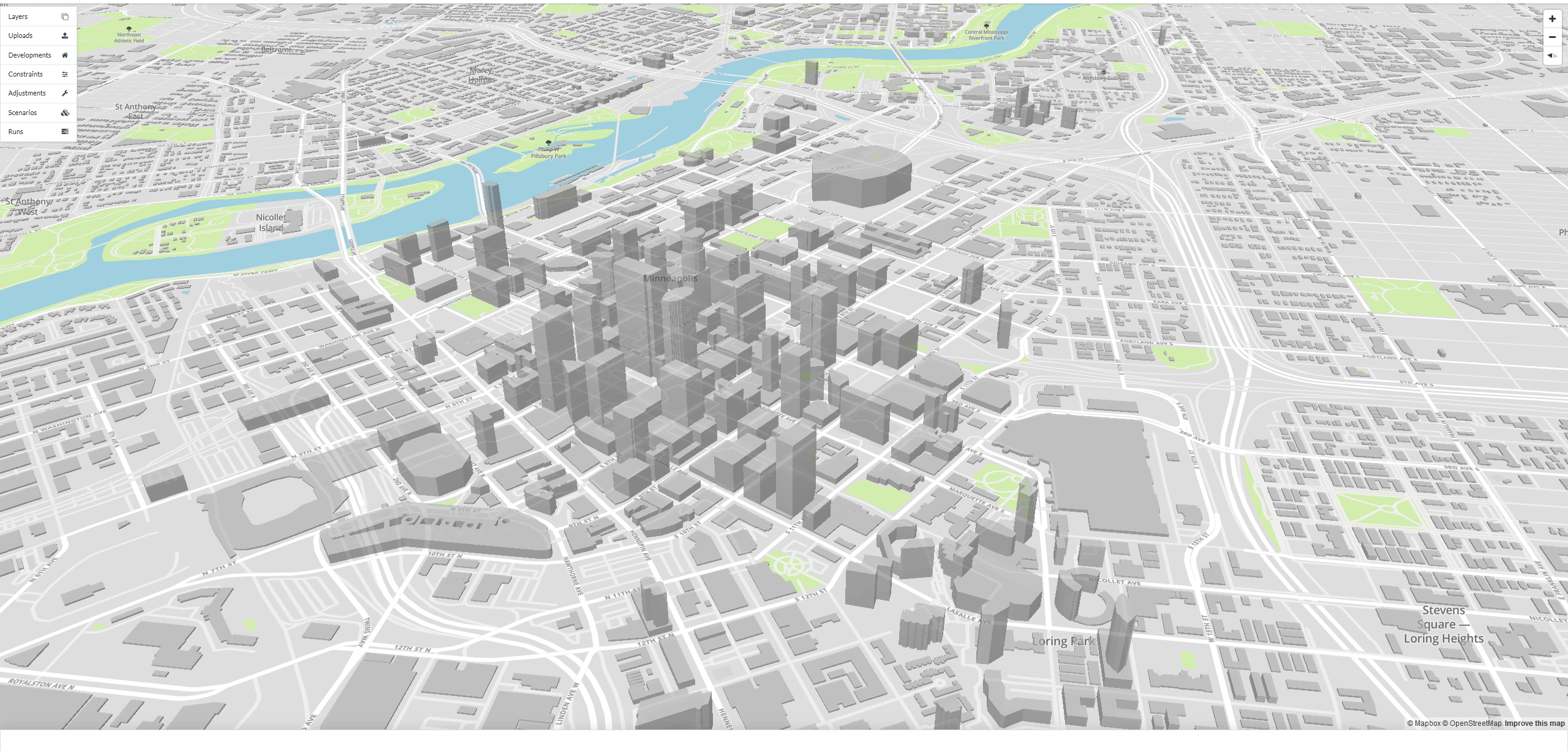
Pan in a north-easterly direction until you arrive over downtown Minneapolis and zoom in. For context, let’s turn on OpenStreetMap (OSM) buildings. Open the layers menu from the toolbar, click the eye icon next to OpenStreetMap Buildings to view buildings available for this area. 3-dimensional buildings will begin to load on the map. Tilt, pan, and zoom to get a good view of the downtown skyline and to become familiarized with the navigation controls.
Now let’s get ready to run our first simulation! A new scenario must be composed so that we have a scenario to simulate. Click the Scenarios button in the toolbar, which will bring up the Scenarios table. This is an empty table, as no scenario has been created yet. Right above the table, click Create Scenario, which will bring up the Create New Scenario form. What you see in this form is all the scenario levers available for composing a scenario using the block-level model template. Macro-level assumptions about demographic, employment, and residential unit growth are in the left half of the form. The right half of the form shows options related to travel model skims, development projects, development constraints, and model adjustments (we’ll cover each of these scenario input types later on). For now, we will compose a simple scenario. Enter a value of 1 for Household Growth Rate, and a value of 1 for Employment Growth Rate. This means that this scenario assumes a 1% annual growth rate for both households and jobs in the region. Enter a value for 6 in the Residential Vacancy Rate field, replacing the default region value. This means that we assume a structural vacancy rate of 6% over the forecast period. Name the scenario Simple Scenario. Click Save to finish creating the scenario, and notice that a scenario record now appears in the scenarios table.
Next, click the Runs button in the toolbar, which will bring up the Simulation Runs table. This is empty, as we have not run a simulation yet. Click on Create New Simulation Run, right above the table. On the left side of the form, select the scenario to simulate. In this case, we have only created Simple Scenario, so click the checkbox next to its name. Enter the year to simulate to. Recall that for the block-model the base-year is 2010, so the simulation end year must be year 2011 or beyond. If you are on a trial account, enter any end-year between 2011 and 2015. If you’re a subscriber, input any end year value up to 2050 (and contact us here if you’d like to simulate past 2050!). Leave the Random Seed field blank for now. This is an optional integer field that allows you to fix the random seed in UrbanSim’s random number generator so as to make simulation results replicable. Leave the Calibrated Coefficients toggle in the on position, indicating that we want to simulate with calibrated coefficients. In general, simulating with calibrated coefficients is the way to go, to better account for observed growth trends. Running a simulation without calibration can be a useful exercise to learn about the full sensitivities of the model, as calibrating to observed data does dampen some of the behavioral sensitivity of the model specification. Next, click Start Simulation to send the simulation request to our cluster of servers.
A new record should appear in the Runs table corresponding to our simulation run. Note the Status field. When this field shows Initializing, the compute resources to run the simulation are being prepared. Starting means that the simulation has been successfully assigned to a machine, and the simulation is reading scenario inputs, loading base data, and setting up the simulation environment. Running means that simulation is in progress. At this point, click on the magnifying glass icon to the left of the simulation run record in the table view. A window appears that allows us to inspect the simulation’s progress. View the progress bar, the current simulation year, and the current model step that is being simulated. After the simulation completes, the View Log button will display the simulation log (this will be empty while the simulation is in-progress), and the Status column in the table view will show Completed. You can download the default set of indicator variables for the simulation for any of the provided geography levels for any simulation year by clicking on the Downloads button.
Congratulations, you’ve run your first simulation! In the layers menu, you’ll find new indicator map layers corresponding to the simulation run. They will be named with the simulation run ID and the geographic level of the indicator layer and will find charts for the simulation under the charts action button. We’ll view indicators in the next chapter.
Chapter 2: Composing complex scenarios and assessing model results
Now that we’ve run a simulation, let’s dive a bit deeper into some of the other features of the platform. At the end of this chapter, we will run a simulation that takes advantage of additional scenario levers.
Let’s change basemaps to switch the contextual information shown on the map. Return to the Layers menu and click on Layers in the toolbar. If the OpenStreetMap Buildings layer is turned on, switch them off by unchecking the eye next to the layer so that we can better see the basemap. Now click on Basemap. Toggle the basemap by clicking the Style dropdown menu. Select Mapbox: Satellite to show satellite and aerial imagery which is useful for viewing what is on the ground. Toggle the Mapbox: Outdoors basemap for a useful view of natural features. Explore some of the other basemap options. See the Layers section of the documentation for additional information.
Let’s upload some control total files as we ready the inputs for composing another scenario. Click on Uploads in the upper right toolbar to bring up the Uploads interface. You will see uploaders for Travel Model Zones, Household Control Totals, Employment Control Totals, Travel Model Skims, Zoning and other files. See the block model upload section of the documentation for additional information on uploading files. For now, we’ll upload Household Control Totals and Employment Control Totals.
Download the following sample files so that you can upload them:
On your local machine, open each of the sample files above (e.g in Excel or in a text editor) to view the control totals. Household Control Totals contain macro-level information on household change in the region, and Employment Control Totals contain macro-level information on employment change in the region. These sample CSVs give, for each simulation year, the total number of households and jobs in the region. These control total tables can be used to evolve households and jobs in detailed ways as well, say by giving household totals by household type, or job totals by employment sector. See the Block Model Data Schema section of the documentation for additional information on how to format files for the Block Model.
In the Uploads interface, click the green + icon to the right of Household Control Totals. In the Name File field, enter Baseline Regional Household Controls. Then click Choose File to identify the file in your local file system, and then click Upload.
Similarly, let’s upload the employment control totals. Click the green + icon to the right of Employment Control Totals. In the Name File field, enter Baseline Regional Employment Controls. Then click Choose File to identify the file in your local file system, and then click Upload.
We now have the macro inputs needed to run a simulation using control total tables. Remember that control totals tables can give the user fine-grained control over how the population of households and jobs evolves in the region over time. We might want to simulate the impact of an aging population for instance, or the expansion of a particular economic sector.
Next, let’s create a development project. Development projects represent known upcoming real estate development projects in your region. The platform’s Developments feature can be used to enter information on the entirety of a region’s real estate development pipeline. But first, we need to create a tag. Tags are groupings of entities, and each development needs to be associated with a tag. Click on Developments in the toolbar, and then click the Manage Tags button at the top of the table view. Then click on the green + symbol to the right of Developments. Give this new tag a name of Baseline, and then click Save. Click Done to exit the Tags window. For more information on tags, see the Tags section of the documentation.
Now that we’ve created a development tag for development projects to belong to, we’ll create the development project. Click on Developments in the toolbar if you are not already there. Then click Add Project to bring up the Create new development project form. Let’s give our new project a name.
In the Name field, enter Nicollet Village. Click Next.
Now let’s site the project. Click on Start selection, which takes you to a map view. Select the block(s) this project will be located on. Just north-east of downtown Minneapolis, notice a prominent island in the Mississippi river named Nicollet Island. Zoom to the island and click on the northernmost block on the island. The selected block turns green. Click Confirm selection. Click Next.
Now let’s select a building type for the project. In the Building type drop-down menu, select Rent Multifamily. Click Next.
Because we have selected a residential building type, we next fill in the Residential units and Average unit size fields. Let’s say this project has 150 residential units and an average unit size of 900 square feet. Note the tenure of the units will automatically populate for the building type, in this case 100% rental units. In addition, it is assumed by default that the project will have 100% market rate units. Click Next.
Now, let’s specify the timing of this project. In the Start year field, enter any year post 2010- let’s give this project a start year of 2014. In the simulation, construction on this project will commence in year 2014. In the Duration field, we specify how long construction will take- populate this field with a value of 24, indicating that construction will take 24 months to complete. Note that once you enter this information, you now have the optional ability to Add development phases to set the timing of when units or space will come on line. Click Next.
Leave the Status of the project as Committed indicating this project will be built with a high degree of certainty.
In the Development tags field, select the Baseline tag we created earlier so we can use this tag that holds this development project in our scenario. Now click Complete to finalize project creation. In the map view, you’ll see a blue polygon representing the location of the project we created.
You’ve created your first development project! In scenarios that include the relevant tag, this project will be inserted into the simulation in the specified simulation year and with the specified characteristics. It’s a good idea to input as many known development projects as you can into the platform so as to supplement simulation results with local expertise on upcoming real estate events. For more information on developments, see the Developments section of the documentation.
Now let’s create a development constraint. Development constraints represent maximum allowable development densities, as prescribed by zoning, development regulations, and natural constraints that limit development. As with developments, start by creating a new constraint tag for constraint records to belong to. Click on Constraints in the toolbar, and then click the Manage Tags button at the top of the table view. Then click on the green + symbol to the right of Constraints. Give this new constraint tag a name of Baseline, and then click Save. Click Done to exit the Tags window.
In the toolbar, click on Constraints. Then click Add Constraint to bring up the Create new constraint form.
Let’s give our constraint a name of TOD Upzone.
Select the blocks that this development constraint will apply to by clicking Select geometry. Click the block on the southern end of Nicollet Island to select it, which will highlight the block in green. Then click Confirm selection, which will bring us back to the form view.
This area is near several existing bus lines and we want to upzone this area to support higher densities to take advantage of its proximity to transit. In the Start year field, enter a value of 2012, indicating that this development constraint will apply from the year 2012 and onwards in the simulation (or until the next constraint year, if multiple constraints exist on the block).
Next, let’s populate the maximum allowable densities associated with this constraint. In the Maximum residential density field, enter a value of 30. In the Maximum employment density field, enter a value of 10. These values mean that development is allowed up to a maximum density of 30 dwelling units per acre and 10 jobs per acre. This will result in an improved capacity of this selected block to hold higher density development. The simulation will respect these upper bounds on development density. If we had entered zeros in these fields, we would have prohibited development entirely on the selected block.
In the Constraint tags field, select the Baseline tag we created earlier. Then click Save to finish creating this new development constraint. You’ll see a red polygon on the map representing the location of our new constraint record. For more information on constraints, see the Constraints section of the documentation.
Now, let’s create a scenario using the new inputs we have created. Click the Scenarios button in the toolbar, which will bring up the Scenarios table. You will see a single scenario in the table, the one we created in Chapter 1 of this tutorial. Right above the scenarios table, click Create Scenario, which will bring up the Create New Scenario form. Name this scenario Baseline. Input a Residential vacancy rate of 6%. In the Household control totals drop-down menu, select the household control totals file we uploaded, and in the Employment control totals drop-down menu, select the uploaded employment control totals file. In Development tags, type in or select the Baseline tag we created earlier, and similarly for Constraint tags type in select Baseline. Click Save to finish creating the scenario, and notice that a scenario record now appears in the scenarios table. For additional information on scenarios, see the Scenarios section of the documentation.
Let’s simulate the Baseline scenario we just created. Click the Runs button in the toolbar, which will bring up the Simulation Runs table. Click on Create New Simulation Run, right above the table. On the left side of the form, select the scenario to simulate. In this case select the Baseline scenario by clicking the checkbox next to its name. Enter the year to simulate to: 2015. In the Random Seed field, enter a value of: 1. Recall that the random seed is an optional integer that allows you to fix the random seed in UrbanSim’s random number generator so as to make simulation results replicable. Click Start Simulation to send the simulation request to our cluster of servers. For additional information on running simulations, see the Runs section of the documentation.
When the simulation completes, view spatial indicators generated by the run. Open the layers menu from the toolbar, click the Add Layer button.
Find the layer in the Available layer list called block indicator run 2 and click the circle next to it to use it and click Next. As the indicator layer naming convention suggests, we’ll view block-level indicators from run ID 2.
Now click on the Field dropdown box to select the type of indicator to visualize on the map and the Year. Select the indicator named Total population accessible within 1.5km along the auto street network (natural log) and the year 2015 and click Next. Note: You also have the option to view this indicator as a time series in the time slider to easily look at values over time.
Now let’s select how we want the data displayed. In the Color scale dropdown menu, select Orange Red and then click Next. The map should start filling in census blocks with colors corresponding to the indicator values. Browse around to get a sense for the spatial variation in local population. More densely populated areas will take on a darker red hue. See the Indicators section of the documentation for further details. Feel free to choose a different indicator to display and try extruding the values.
Now let’s look some of the charts generated by the simulation.
Click on the Runs menu button and put your cursor over the blue action button for run ID 2 and click on charts.
A pop-up box will appear on the map with a dropdown box with a selection of default charts exported by the simulation. Select one to view it.
Close the chart box by clicking the red x button.
Now let’s look at the simulation results exported as data tables.
In the Runs menu, put your cursor over the blue action button for run ID 2 and click on status.
A pop-up box will appear with information on the run status with a menu to show logs and a menu for downloads. Click on downloads and select the county level option and the file for 2015 CSV Indicators.
The file will download to your machine and you can open the file in any spreadsheet or GIS application to further explore the raw indicator results.
Chapter 3: Collecting and incorporating stakeholder feedback
Now that we have launched simulations and explored the results, let’s look at some of the features available to incorporate feedback into the modeling process.
First let’s use a hypothetical example: Staff at your organization or external public officials have assessed your model results and would like to provide feedback for consideration to improve the input data utilized by the model. Specifically they suggest that the 2010 jobs base data counts for the Census blocks representing the Minneapolis–Saint Paul Joint Air Reserve Station are underrepresentative of the large number of military jobs located there and should be updated with new job counts.
Let’s create a new comment to represent this feedback. Comments can be used to gather and manage feedback from stakeholders at any point in the modeling process. Open ended comments can be created and managed in UrbanCanvas and associated with a location on the map.
Navigate over to where the Minneapolis–Saint Paul Joint Air Reserve Station is located. To do so, type in Minneapolis−Saint Paul International Airport into the search box and click on the first option in the dropdown. The map will pan you to the geocoded location.
Now let’s find the Census block that corresponds to the area we want to associate with the feedback. Type in the search box: geom:270539800001033 to search the base data Census blocks for this ID and the map will pan over to the block centroid.
Turn on comments by clicking the comment icon in the UrbanCanvas header to the left of the Uploads button. This will toggle comments on and off the map.
Create a new comment by clicking the create comment icon underneath the right-side map navigation icons and click and drag the red comment marker to the center of Census block 270539800001033 then confirm the location by clicking the confirm comment location icon.
Type in the feedback for this comment in the text box inside the comments panel. Click add comment to save the comment.
You now have an open comment on the map at this location representing the feedback that can be used to track how its addressed. For more information on comments, see the Comments section of the documentation.
Now let’s address this comment by creating an adjustment record to assert a new jobs number at this location. Alternatively, in a situation like this the base data itself could be updated directly, however for the purposes of this tutorial we will be using an adjustment. Adjustments override simulation results in user-defined locations. This can be useful for areas such as military bases and universities, where non-market processes dictate what will occur. Adjustment records can then be tracked in a transparent way over time. As with developments and constraints, start by creating a new adjustment tag for adjustment records to belong to. Click on Adjustments in the toolbar, and then click the Manage Tags button at the top of the table view. Then click on the green + symbol to the right of Adjustments. Give this new adjustment tag a name of Feedback, and then click Save. Click Done to exit the Tags window.
Click Add Adjustment to bring up the Create new adjustment form.
Let’s give our adjustment a name of Minneapolis–Saint Paul Joint Air Reserve Station.
Select the block where the comment is located to apply the adjustment to by clicking Select geometry. Click the 270539800001033 block to select it, which will highlight the block in green. Then click Confirm selection, which will bring us back to the form view.
In the Start year field, enter a value of 2010, and leave the End year field blank, indicating that this adjustment will apply from the year 2010 and onwards in the simulation (or until another adjustment replaces this one, if multiple adjustments exist on the block).
Next, let’s populate the logic of the adjustment. Check the Employment attribute option and enter 800 into the Target Quantity to Match field. Leave the filter options blank. These settings mean that jobs for this block will be forced to equal 800 during the time range specified and will not be impacted by the simulation. Alternatively the filters could be used to assert specific values that match a particular condition.
In the Adjustment tags field, select the Feedback tag we created earlier. Then click Save to finish creating this new adjustment. You’ll see a green polygon on the map representing the location of our new adjustment record. For more information on adjustments, see the Adjustment section of the documentation. This adjustment can be used in a simulation by specifying the Feedback tag when creating a scenario.
Now that we have addressed the feedback in the comment, let’s respond to the comment to update its status.
With the comments tool turned on, click on the existing blue comment icon to show it in the comments side panel and then click on the comment card in the side panel to reveal it.
Enter a reply in the text box under the comment that signals it has been addressed by creating an adjustment record for it. Click on add reply to save the reply.
Mark the comment as resolved by clicking on the three dot icon on the upper right hand side of the comment card and selecting resolve comment.
The comment’s status will change to resolved and the icon will change to a grey color.
Now that we’ve explored some of the platform’s features, you are on your way to becoming an UrbanSim modeler. If you have not already, perusing the rest of the documentation is a good next step or viewing our Planetizen courses. Happy modeling!